5. FasterRCNN In DLP
DLP uses the implementation of FasterRCNN with ZF and VGG16 as base/pretrained networks.
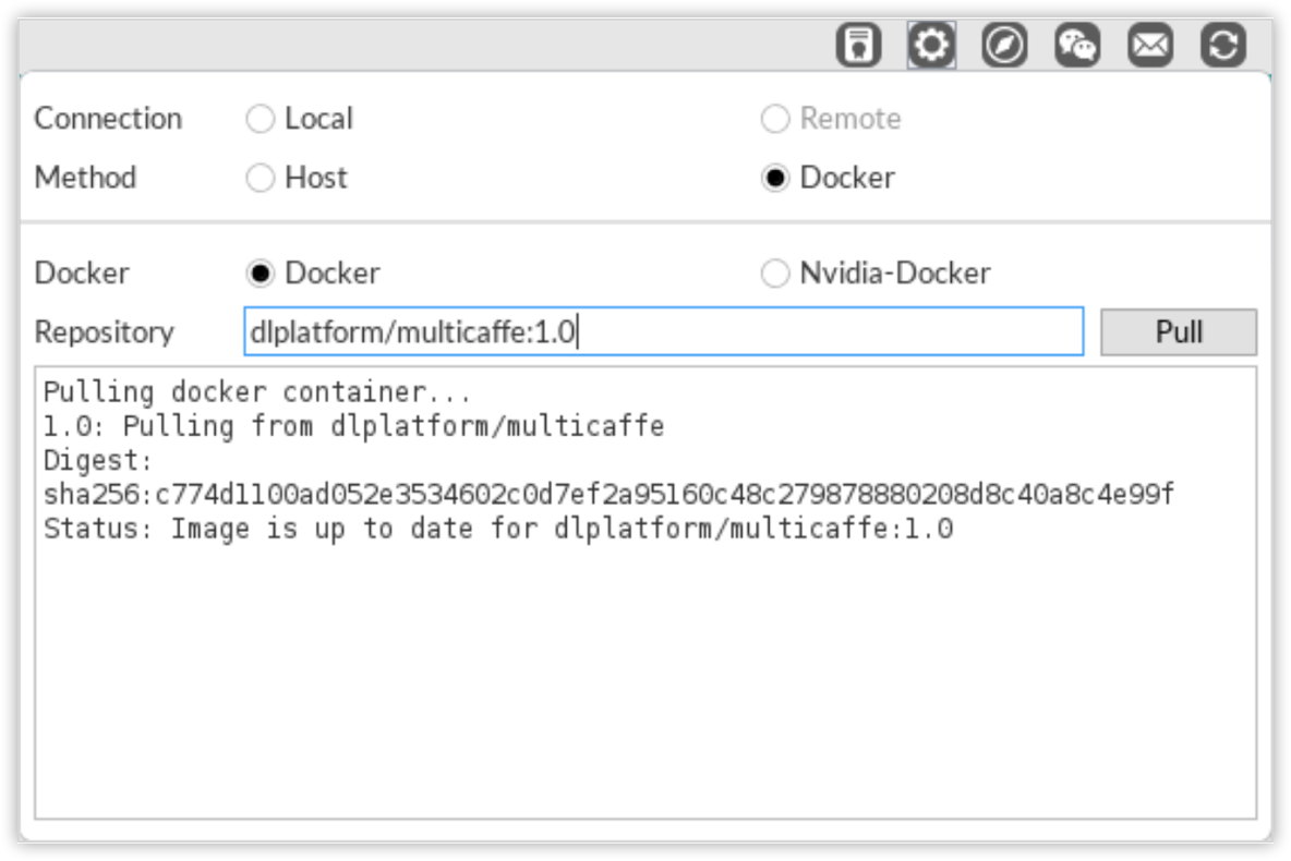
We will build our person/basketball detector using FasterRCNN-ZF because of the simplicity of the architecture. Therefore ZF network will be our base model. You can download a pretrained ZF net specifically designed for this task here.
The remaining of this section is divided in two parts : in the first part, I will illustrate how to train your dataset using FasterRCNN, assuming the images and annotations files are ready. In the second part, I will explain how to annotate your own images for detection in DLP and use the annotated dataset to build a custom object detector.
Part 1. Basketball Detection
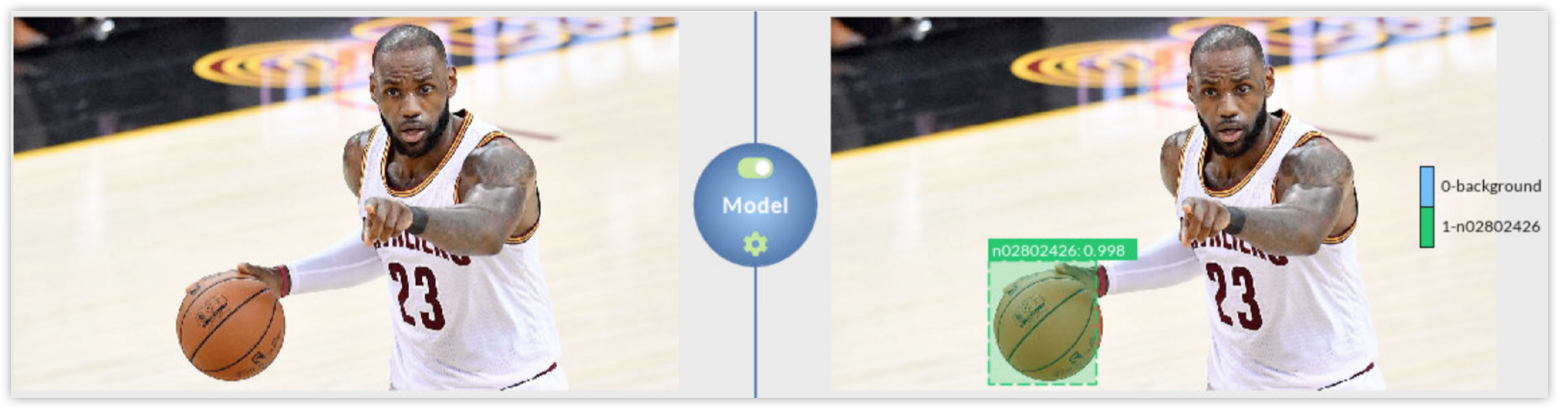
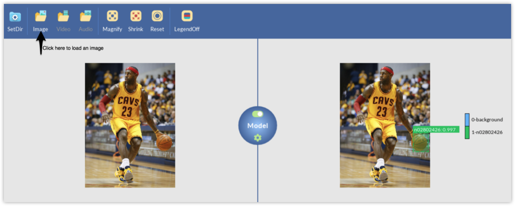
In this part, basketball detection will be used as an example. By the end of this part, you will be able to use a single color image as the one on the left and produce a labeled output like the image on the right.
Download Dataset
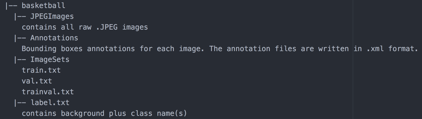
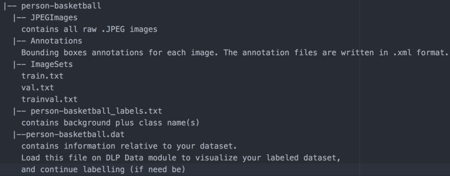
The dataset used in this part is downloaded from ImageNet. Here we provide a link to download the basketball dataset. Once you have downloaded the dataset, you can unzip it into your project directory. The dataset should have the following structure:
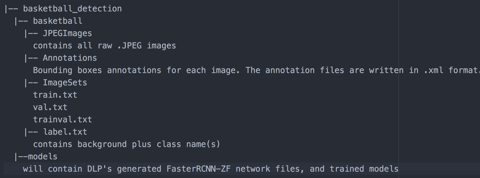
And your project directory should look like this:
Prepare Network
By convention, if you have n classes (n objects of interest) in your dataset, consider it a (n+1)-detection task where the extra class is the background that typically represents each object that you have not defined as object of interest. In this example of basketball detection, since we only have 1 object of interest (basketball), our basketball detection task is therefore a 2 objects (background included) detection problem.
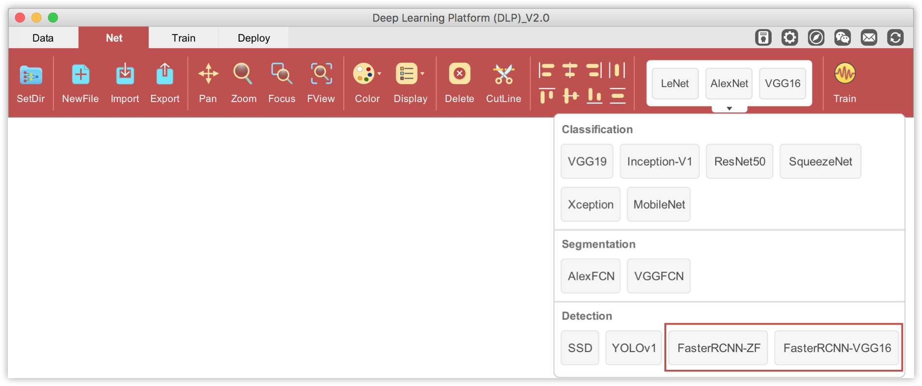
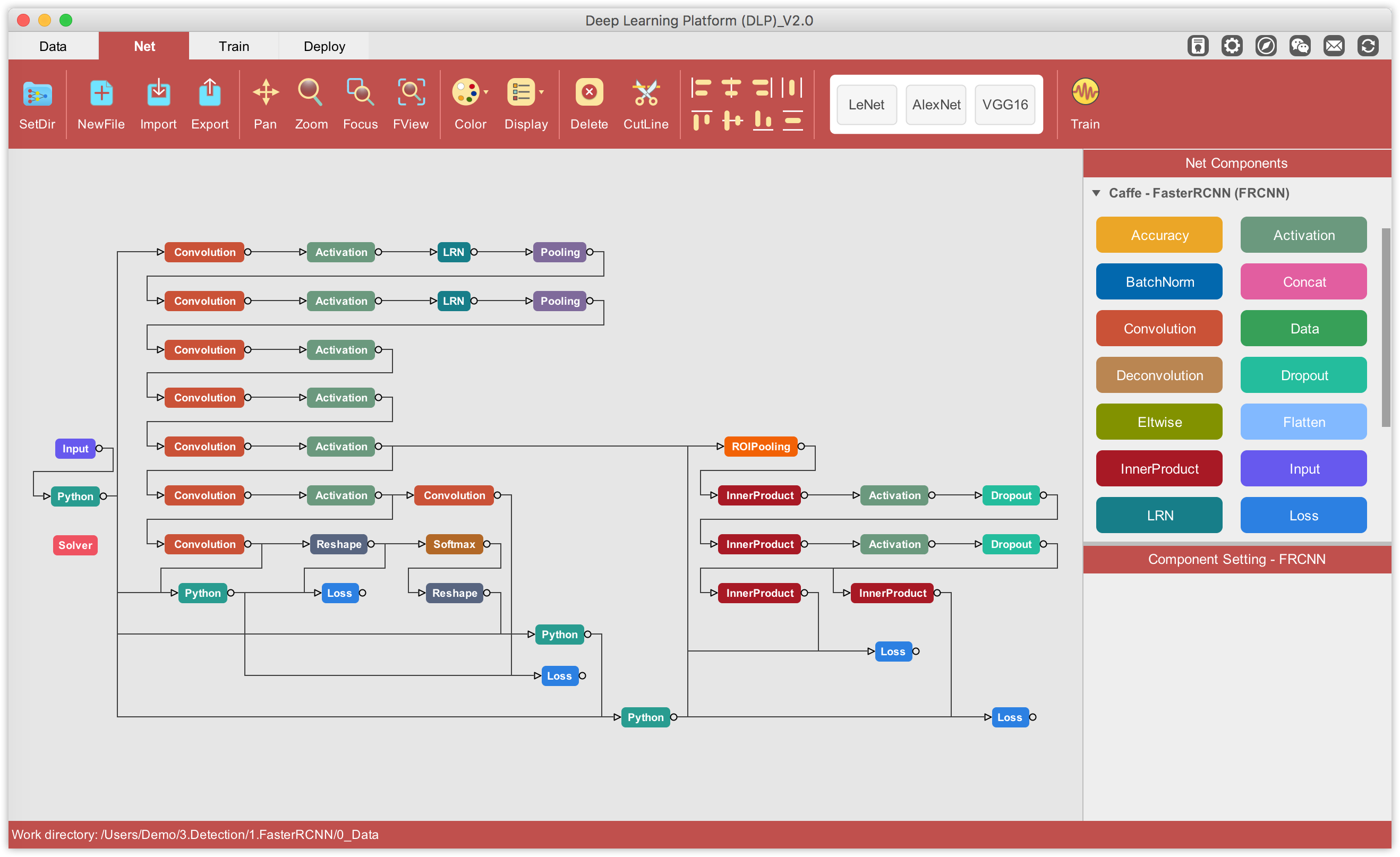
That said, it is time to define/modify some default FasterRCNN-ZF configurations to fit our binary detection task, the goal being to detect a basketball object (named n02802426) in an image. On DLP, drag the FasterRCNN-ZF component and drop it into the visualization area.
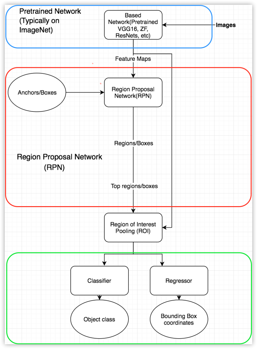
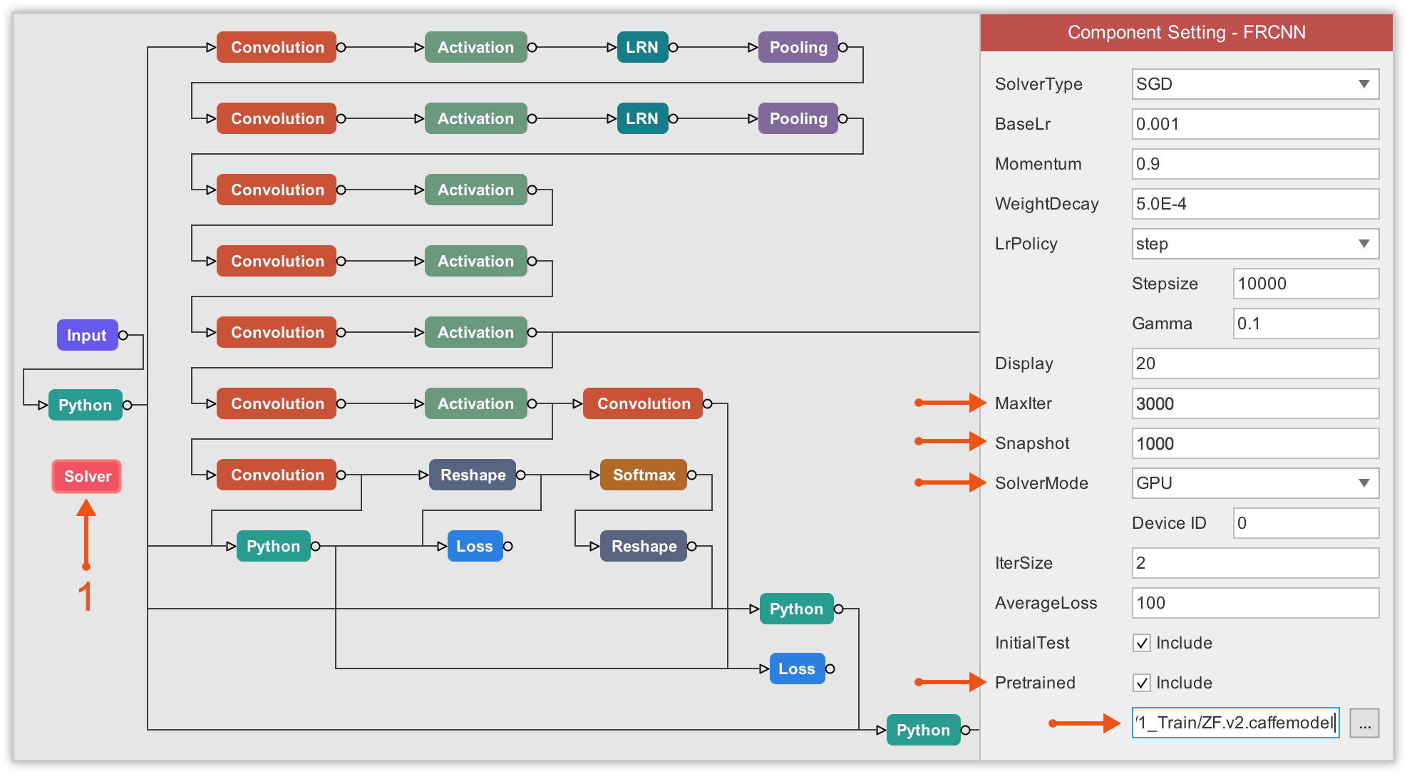
Visualizing FasterRCNN-ZF on DLP, you can easily and certainly better understand the workflow of the algorithm. If you are familiar with ZF-net, you can easily dissect the 3 main components of FasterRCNN as described in section III of this tutorial, namely a base network (ZF-net in this case) responsible for producing feature maps of input images, the RPN net that runs anchors on each spot of feature maps generated by the base network to rank regions/boxes and output the ones most likely to contain objets, and a classification/regression network that uses RPN region proposals to output object class and the associated bounding box coordinates.
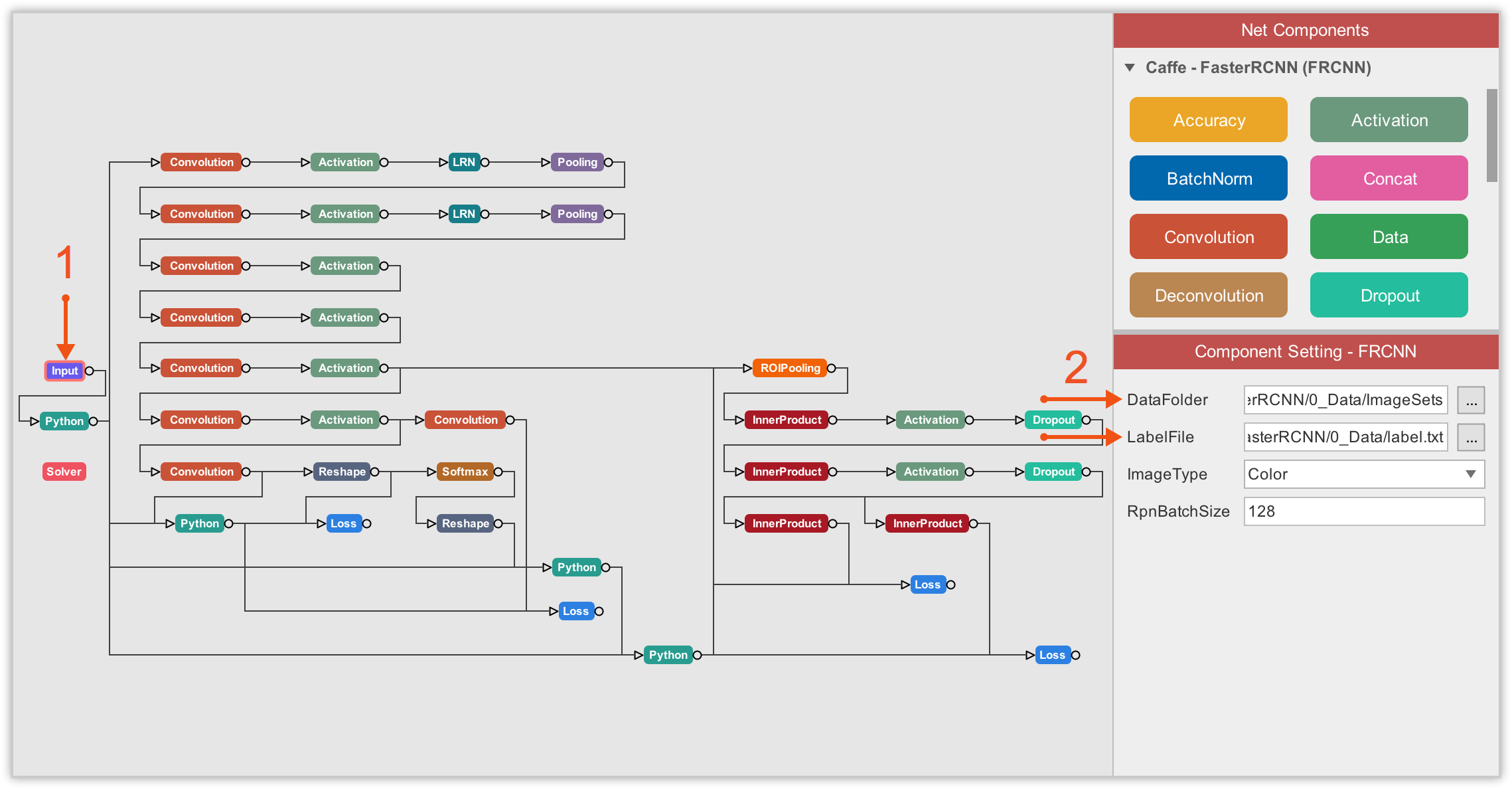
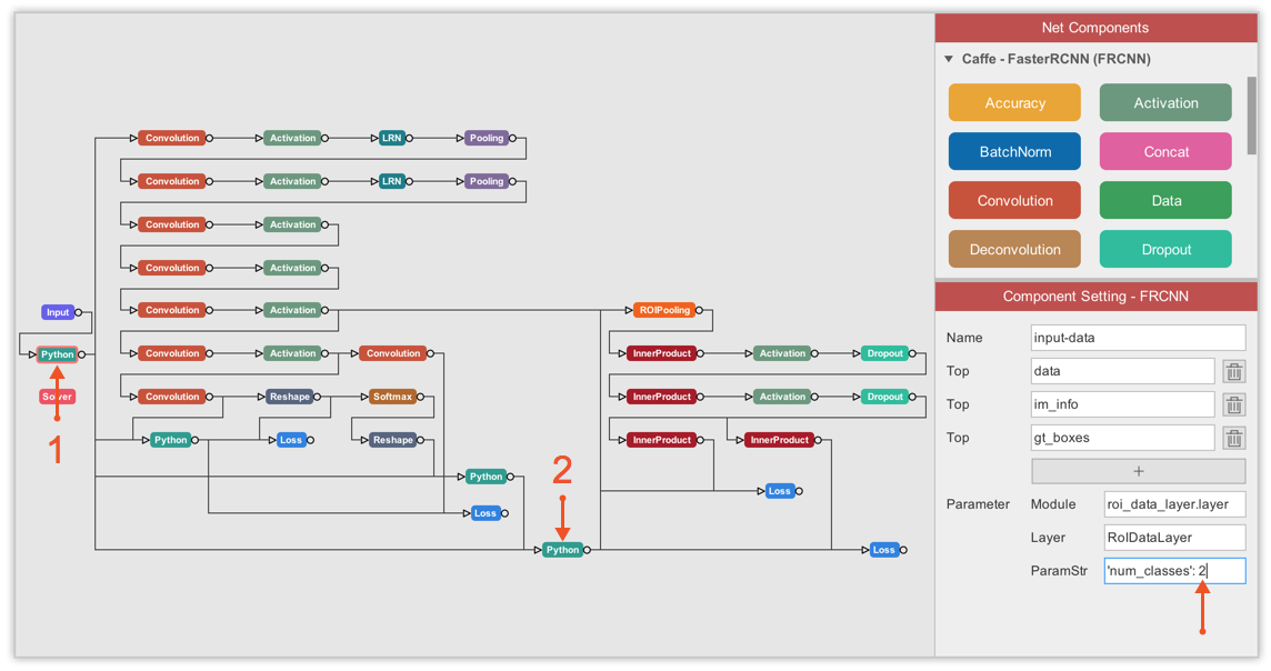
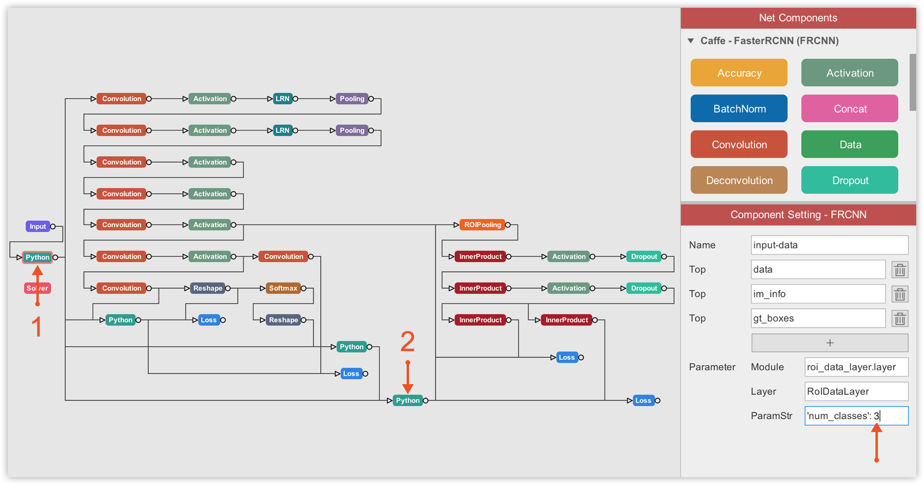
You can configure and/or inspect each layer of the network simply by clicking on the associated component. The configuration associated with the component you clicked will then show up in the Component Setting panel, as illustrated below.
The first thing to do is tell FasterRCNN-ZF where to get the training data. And this is done under the Input component of FasterRCNN. There, you must specify the path to your image dataset folder, and to the .txt label file corresponding to your dataset.
Then, we must update the number of classes in the ROI data layer to 2 because we only are dealing with 2 classes (background and basketball).
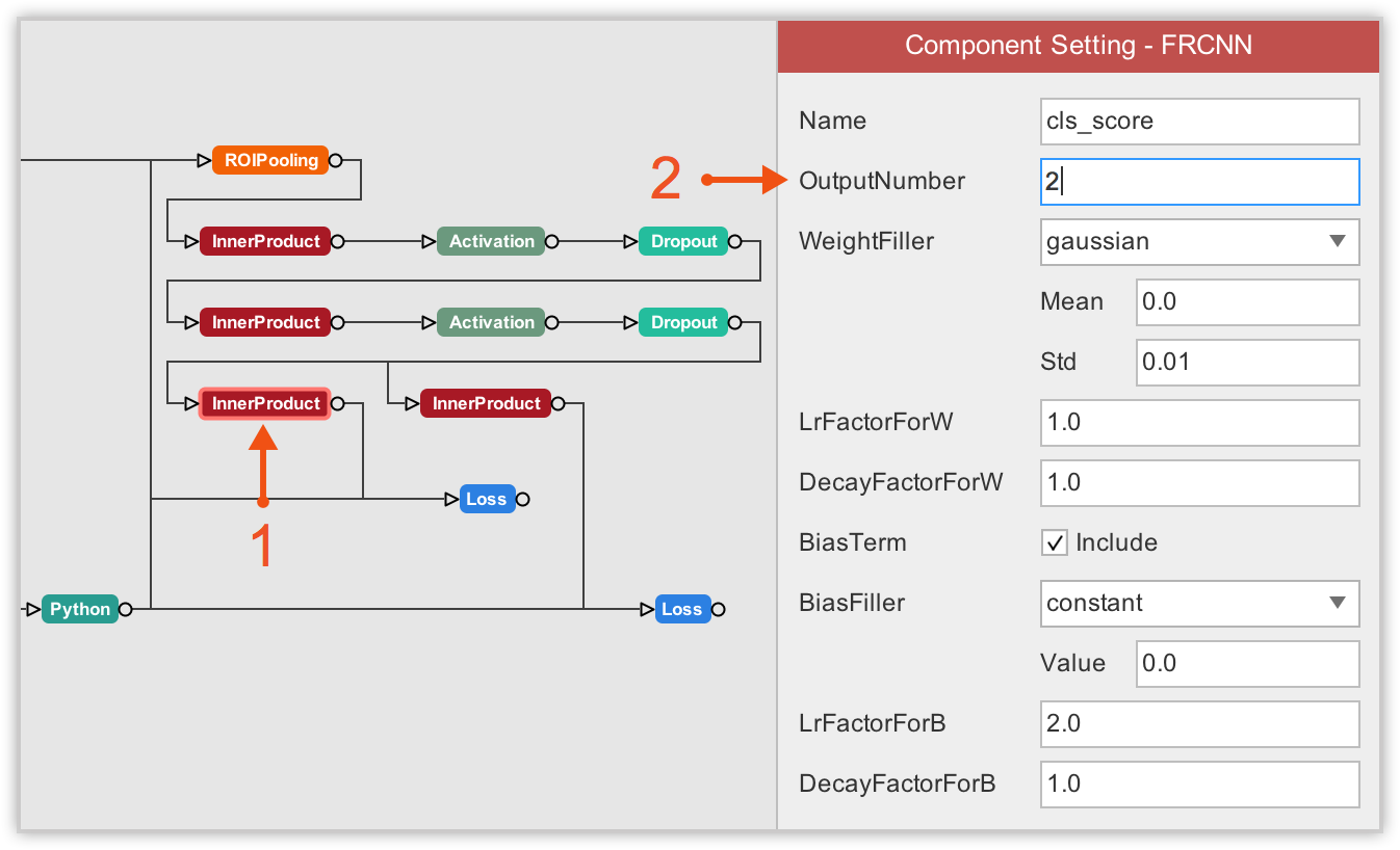
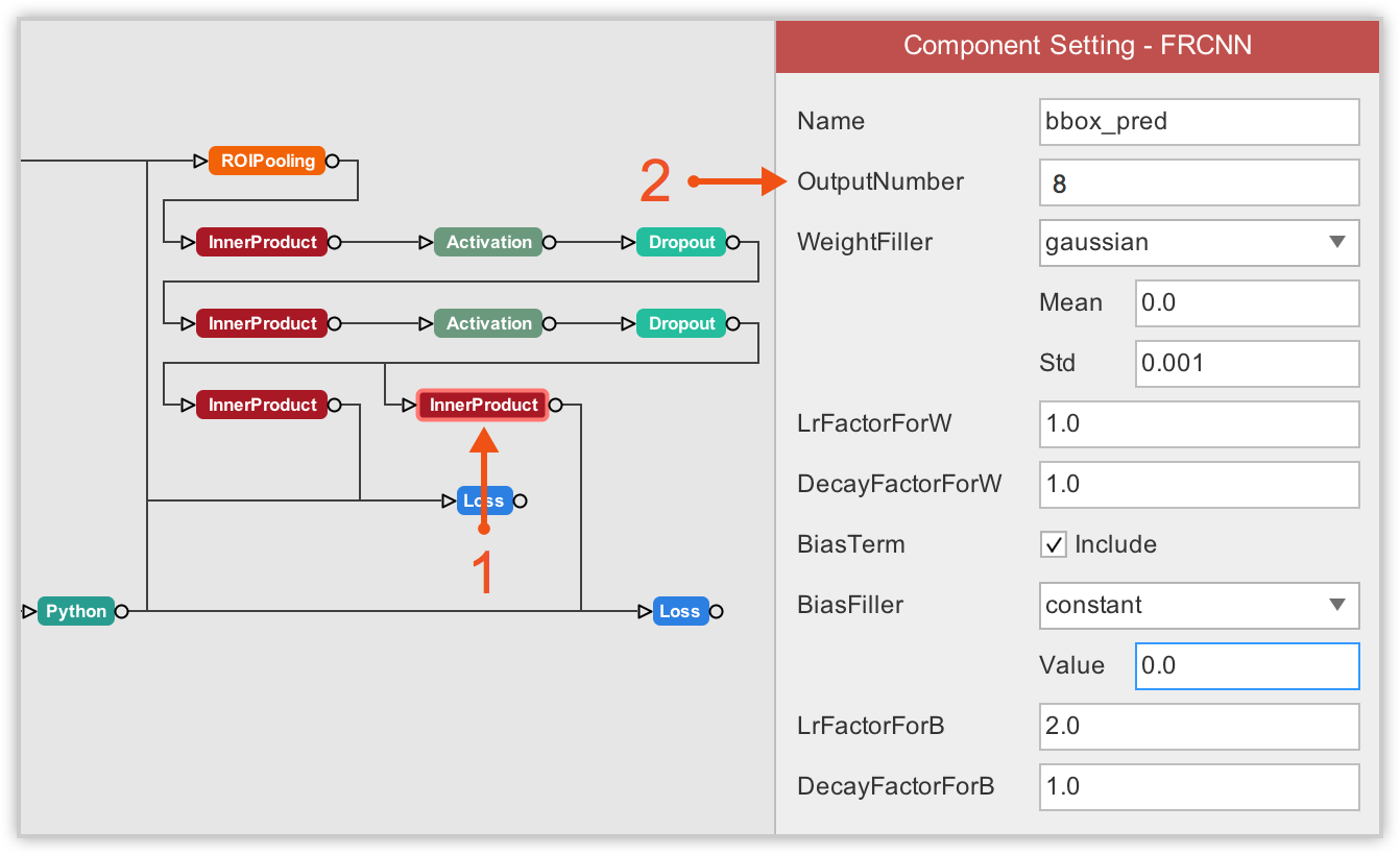
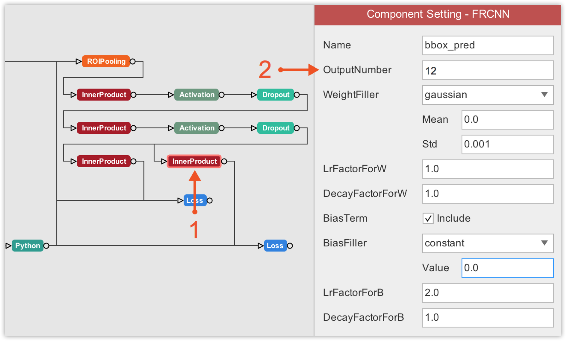
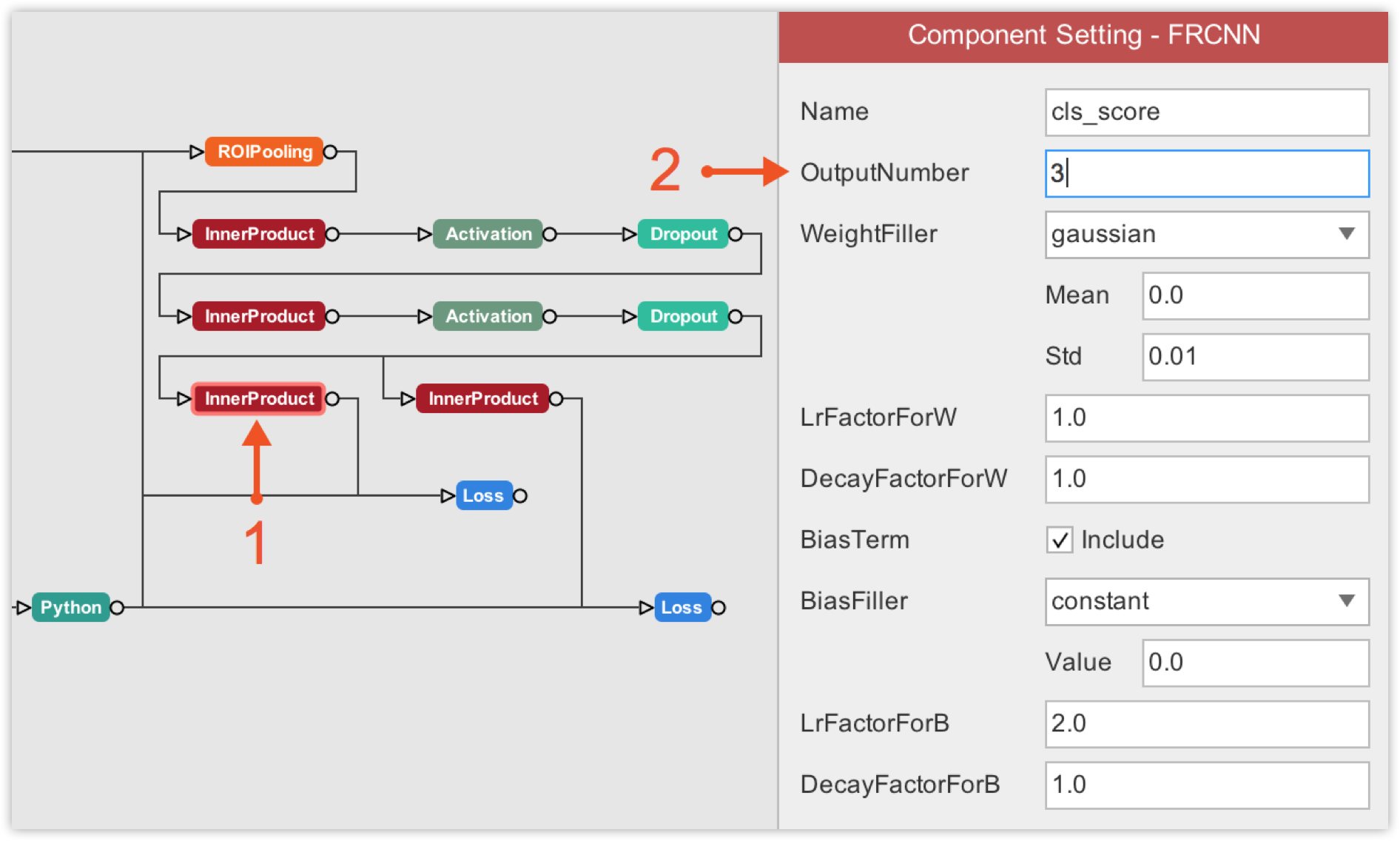
Next, we must update the number of output in final layers. One final layer outputs object classes, so we must update its number of output to 2 because we only have 2 classes (including the background). The other final layer outputs bounding box coordinates for each class, so its output number must be 8 which corresponds to 4 bounding box coordinates * 2 classes.
Finally, we need to configure the Solver component. Here, the most important property of the solver component to which we must pay attention to is the Pretrained. There, we have to load the pretrained model by specifying the path.
Then we can consider properties like the maximum number of iterations (I ran for 2,000 iterations), when to save a snapshot of the model (I choose to save for every 1,000 iterations), and the SolverMode (you must select GPU).
We are now all set to begin training our model. Click on the Train button in the upper-right corner of the window. You will be asked to choose a folder in which to save your network configuration files. This is where your snapshots (models) will also be saved.
Model Training
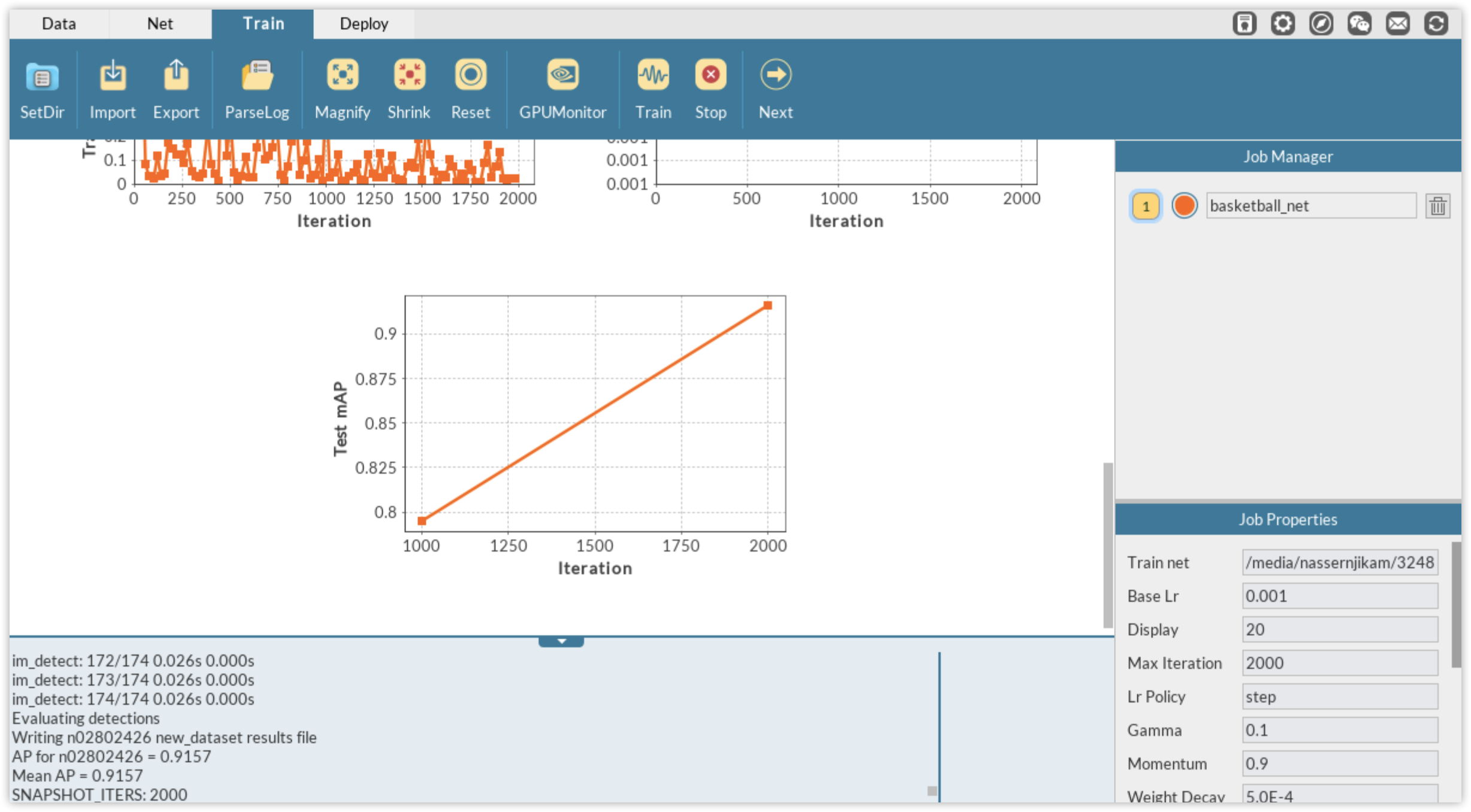
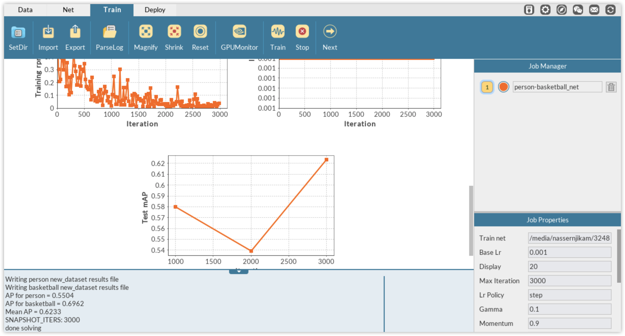
You will then automatically be directed to DLP Train module where you can monitor the training process via different plots or through the log panel. Of all, the most important information to monitor is the mean average precision (mAP) herein computed on the validation set. mAP is the metric used to evaluate the performance of detection algorithms. In DLP, for FasterRCNN, this metric is calculated each time a snapshot of the model is performed. Since we have defined the solver so that we train for 2,000 iterations and take a snapshot of the model every 1,000 iterations, the training is evaluated twice via the mAP calculation.
It can be seen that after 1000 iterations, the mAP score on the validation data is greater than 78% and climbs to more than 91% at iterations 2,000. We will therefore use the second model for inference on unseen dataset.
Model Inference
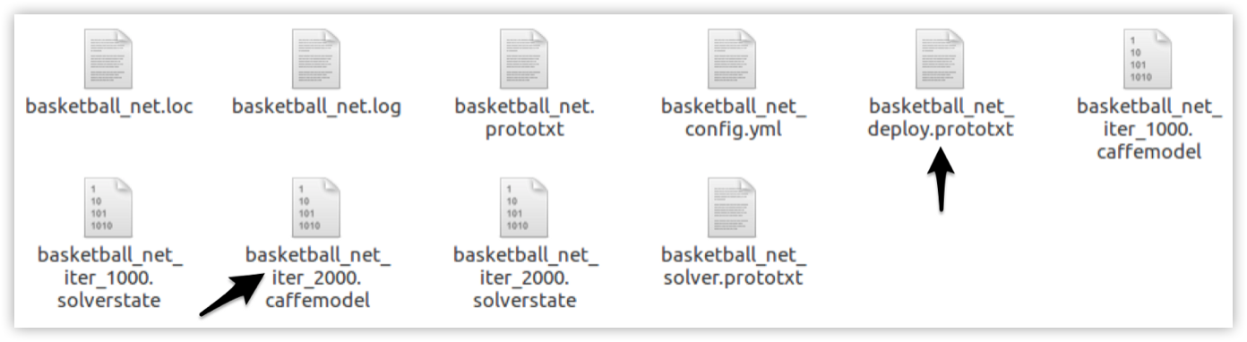
During training, models are saved as .caffemodel file within the folder you have selected to host the network configuration files. This folder should looks like the following after the training:
The .caffemodel obtained after training for 2,000 iterations, and the _deploy.prototxt file generated by DLP in the previous step are both needed, in addition to the label.txt file, for inference.
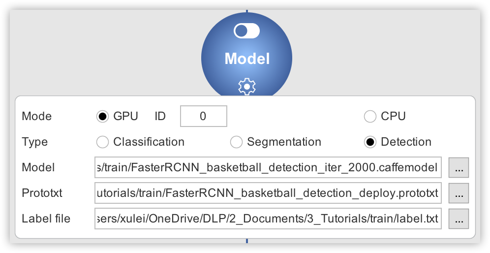
We will now do inference on a couple of images downloaded from the internet using our trained model. Click Next or on the Deploy tab to move to DLP Deploy module. Then click on the dropdown button where you will see the options to configure. Under the mode option select GPU (and corresponding GPU ID if necessary), and then choose the type of inference you would like to perform (detection in this case).
Afterward, fill in the detection model (.caffemodel), the deploy.prototxt file, and the label.txt file in their respective fields. Then the dropdown button will turn green to indicate that the inference engine has all the required files and can now be activated.
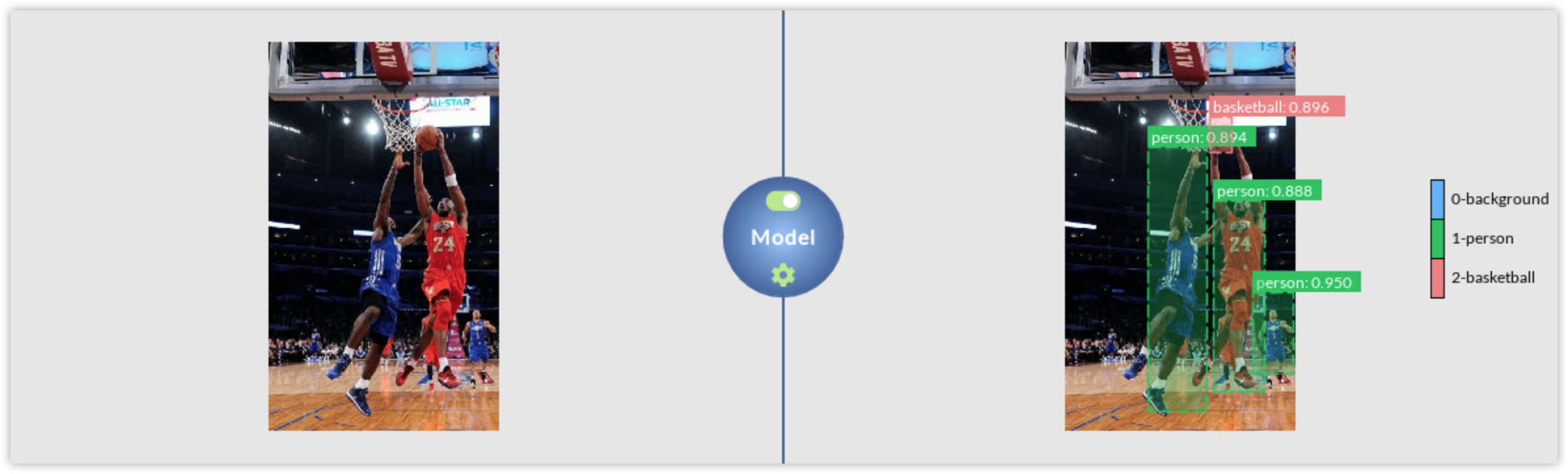
Turn on the toggle button to start the inference engine. You can check whether everything went well by expecting the log panel output. All that remains is to load an image like the one on the left, and DLP will use your trained model to produce a labeled output like the image on the right.
Part 2. Person/Basketball Detection
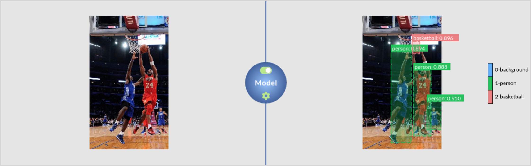
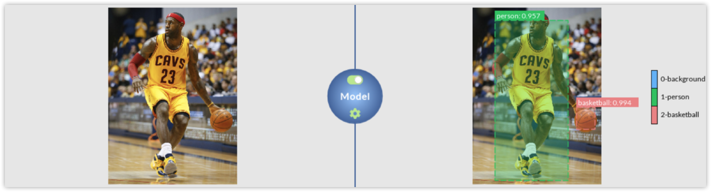
In this part, person/basketball detection will be used as an example. By the end of this part, you will be able to annotate/label your own unlabeled image dataset for detection.
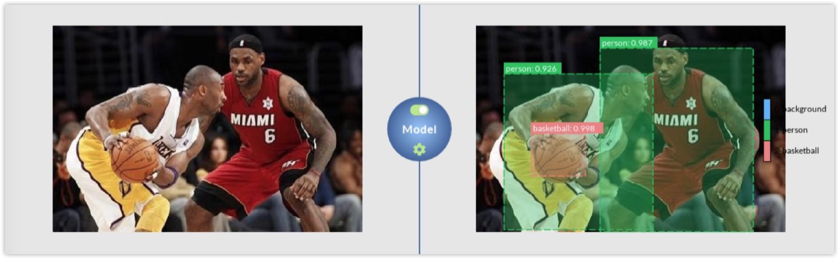
Use FasterRCNN to train on it, and take a single color image as the one on the left to produce a labeled output like the image on the right.
Download Dataset
The dataset we will work with in this part is a small subset of the basketball dataset used above. Typically we randomly selected 98 raw images from the JPEGImages folder of the basketball dataset, and that’s it. We do not need the associated annotation files to those images as we are going to label the data ourselves using DLP built-in image annotation tool. The folder containing the 98 raw images we randomly selected from the basketball dataset can be found here.
Image Annotation/Labeling For Object Detection
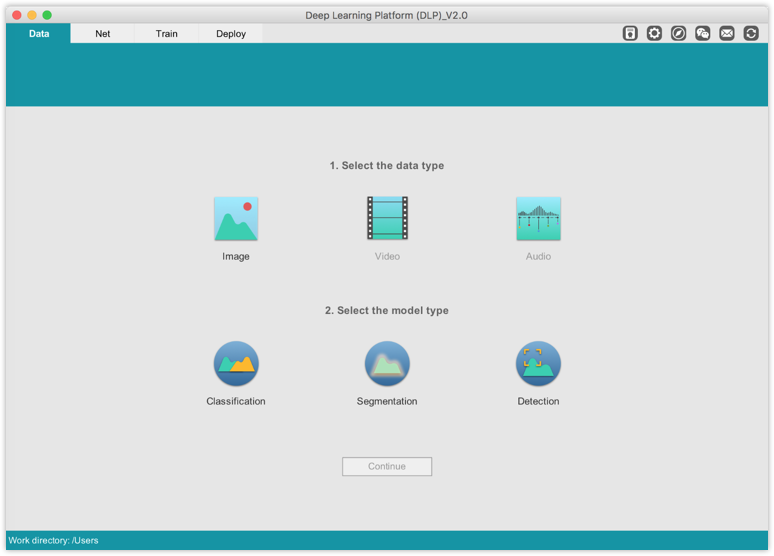
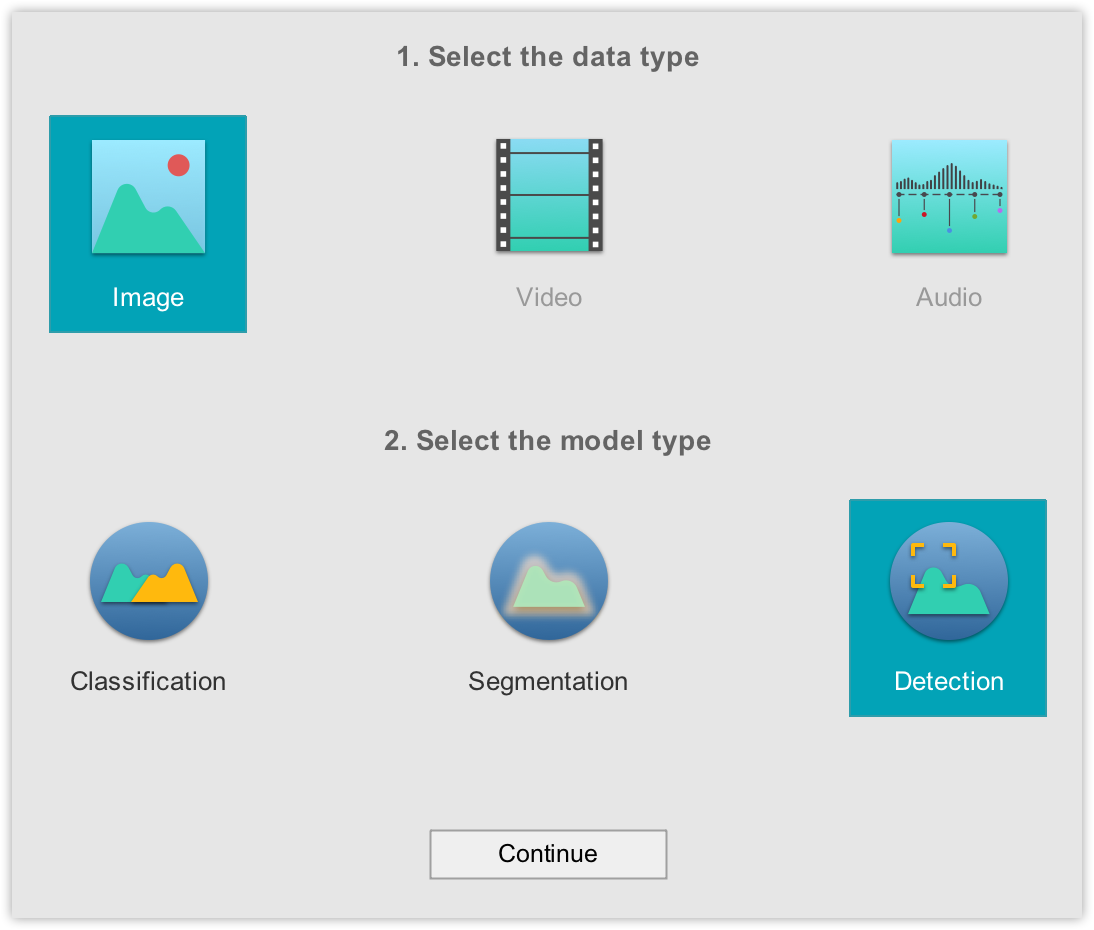
Labeling dataset for object detection consists in drawing bounding boxes (rectangles) around each object of interest in each image in your dataset. In DLP, to start labeling for object detection on your own image dataset, make sure you have selected Image under the 1. Select the data type and Detection under the 2. Select the model type.
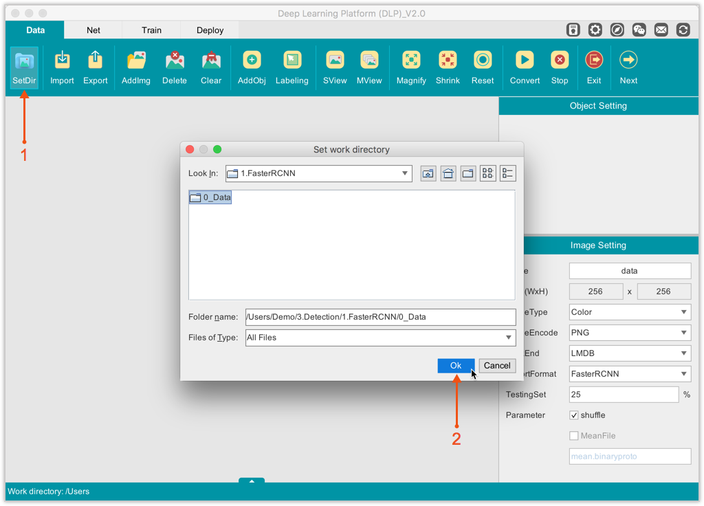
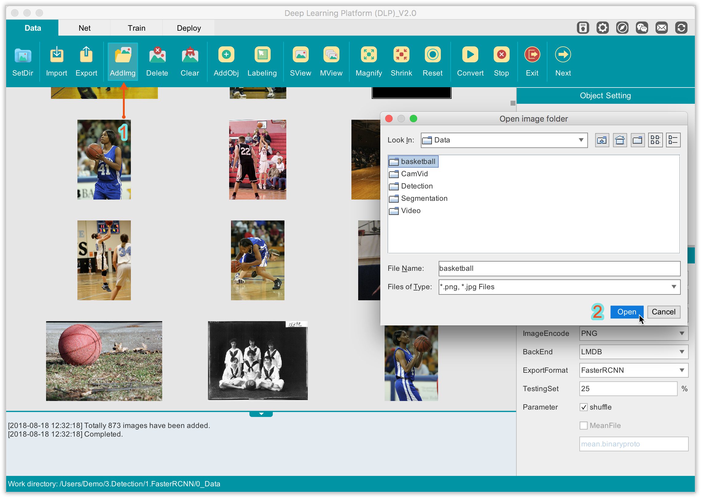
The Data module will be our playground, so be sure you are in this module. Then, on the Function Bar, click AddImg and navigate to the folder containing your raw images to load your dataset into DLP.
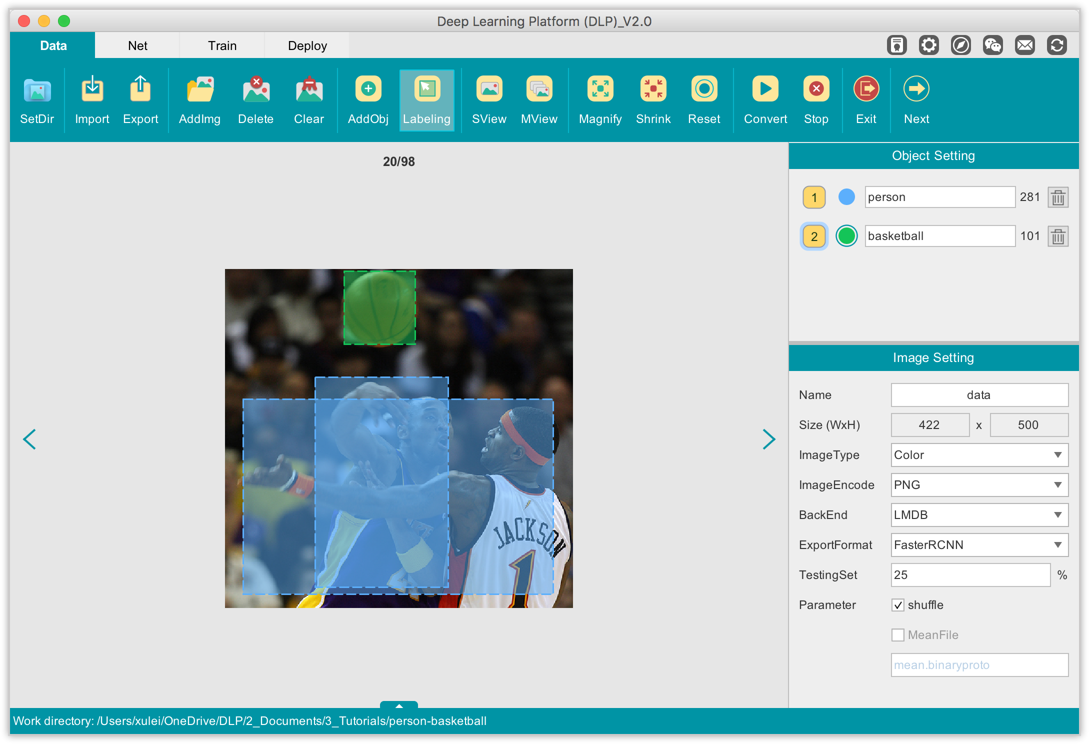
From the visualization area, you can inspect your images, add in more images, delete images, and more. Before we start labeling our images, we must first define our objects of interest. For this example, our objects of interest are person and basketball. To define them in DLP, on the Function Bar, click on AddObj to add an object that you can inspect in the Object Setting panel on the right. By default, the objets of interest are named respectively Object-1, Object-2. You can edit each to give it a more meaningful name.
On the image click to begin drawing bounding box (rectangle) around an object and click again to complete the drawing. If you want to delete an unwanted bounding box, just right-click on it and a Delete option will appear to allow you to delete that rectangle.
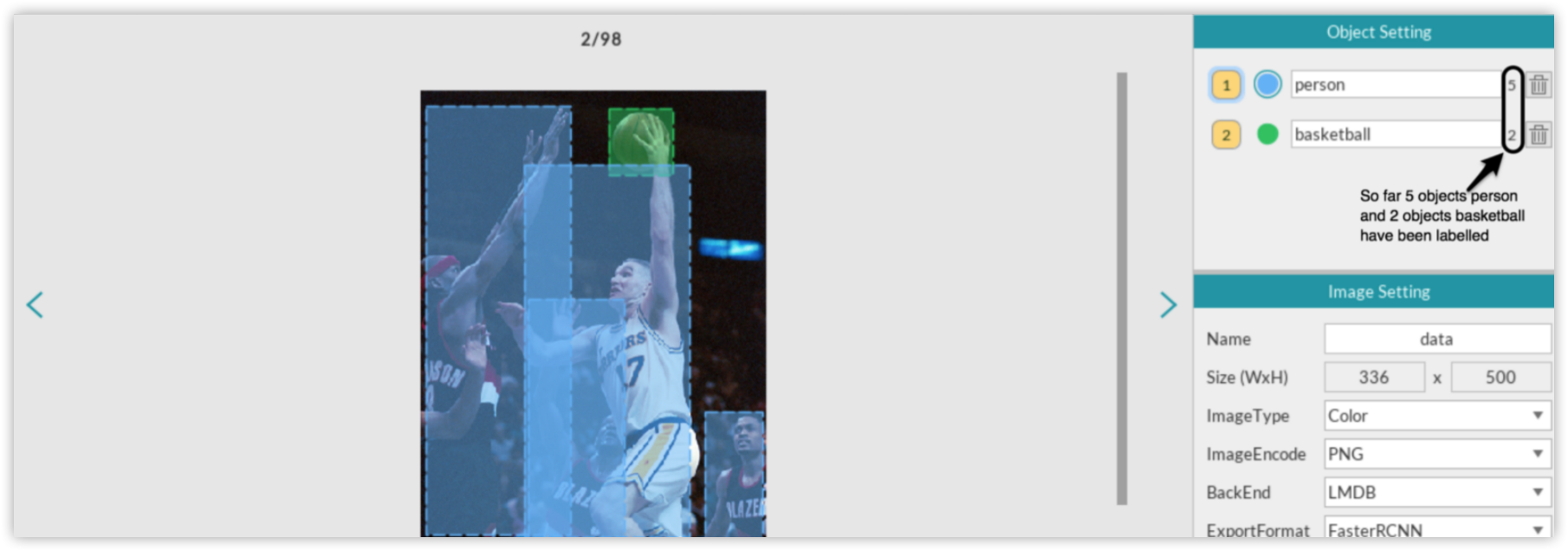
As you progress through your labeling task, you can always check how many objects (not images) have been labeled so far for each object category.
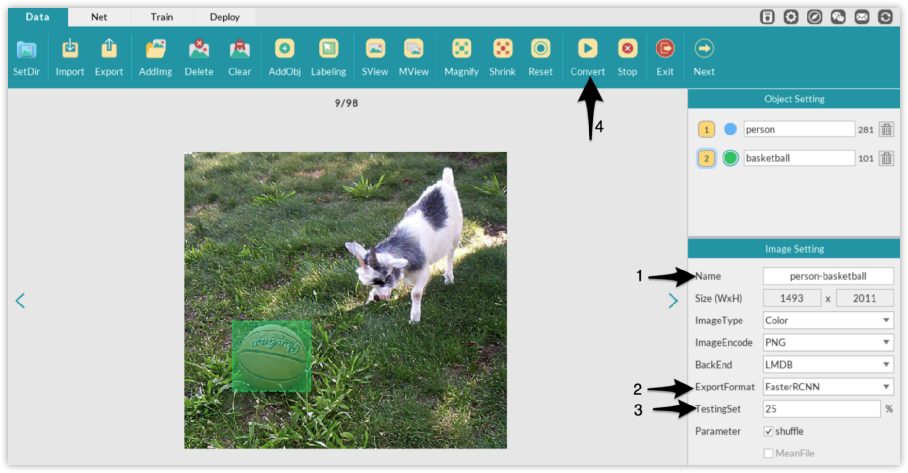
You have probably noticed the Image Setting panel just below the Object Setting panel. It is primarily used to define certain properties that will be used when you are about to export or convert your dataset after you finish labeling. The properties you will most likely be concerned with are the name you wish to give to your labeled dataset, the format in which the dataset will be exported/converted (note that you have options between FasterRCNN, SSD, and, YOLO formats), and the percentage split for the test set. For this example, since we are building a person/basketball detector using FasterRCNN, this is the format we will select when exporting our labeled dataset.
The converted labelled dataset should have the following structure:
As it can be seen, the structure of DLP generated labeled dataset is very similar to that of the basketball dataset we explored in part 1, with the exception of the .dat file which is essential for loading our dataset into DLP and to continue labeling where we left off the last time (by either adding new images to label or continuing to label unlabeled images). You can download the annotated person/basketball dataset in here.
Prepare Network
This process is very similar to what we did with the basketball dataset, except that we now have 3 classes (background included) instead of 2. This implies that the number of classes in the ROI data layer must be updated to 3.
The same is true for the number of outputs of the final layer that produces the object classes, which must also be updated to 3. Likewise, since we now have 3 objects, the other final layer that produces bounding boxes coordinates for each class must now have its output number updated to 12, corresponding to 4 bounding box coordinates * 3 classes.
Next, you have to specify the path to your image dataset folder, and to the .txt label file (person-basketball_labels.txt in this case) corresponding to your dataset. Of course this is done within the Input component of the network.
Finally, I will use the same Solver configuration as the one used for the basketball dataset, do not forget to fill in the Pretrained property with the path to ZF net, with the only exception that I will now set the maximum number of iterations to 3,000 instead of 2,000 used for the basketball dataset.
Model Training
Training on such a small dataset, FasterRCNN-ZF model can achieve over 62% in mAP score after just 3,000 iterations. Not sure whether training for a bit longer might improve the result, but annotating/labeling more images will definitely drastically improve it.
Model Inference
There are three files needed to perform inference for detection on the Deploy module, namely a .caffemodel, a _deploy.prototxt file, and a _labels.txt file.
PS: DLP automatically creates the deploy.prototxt file and .caffemodel during the training process. The _labels.txt model, on the other hand, is automatically created only if you have annotated and converted your image dataset in DLP. Otherwise, you will have to manually define the .txt file.
Turn on the toggle button to start the inference engine. You can check whether everything went well by expecting the log panel output. Subsequently, load an image like the one on the left, and DLP will produce a labeled output like the image on the right.